Reimagining Physics — Part 7
The Reality of Time and Change — Part 1
Physics’ Timeless Universe — Part 2
A Thermocontextual Perspective — Part 3
What is Time? — Part 4
Wavefunction Collapse and Symmetry-Breaking — Part 5
Entanglement and Nonlocality — Part 6
The Arrow of Functional Complexity — Part 7
The Arrow of Functional Complexity
The universe evolved from an initially homogeneous and featureless state to the rich complexity of molecules, planets, and galaxies that we see today. In our own corner of the universe, simple chemicals spontaneously organized themselves into self-replicating forms within as little as 0.1 billion years after formation of the earth’s oceans, and life took off. We see the arrow of evolution in the fossil record and in the advances of civilization, technology, and economies. Despite its overwhelming presence, however, there is no fundamental explanation for the well documented tendency of open systems, sustained by external energy sources, to spontaneously organize complex structures.
In previous parts, I focused on states and their transitions. In Part 7, I shift from states to non-equilibrium systems and their dissipative processes, based on an article published in 2023 [1]. That article establishes a physical foundation for nonequilibrium systems and their process of self-organization into increasingly complex dissipative structures.
Dissipative Processes
The Thermocontextual Interpretation (TCI) [2] establishes the Second Law of thermodynamics and dissipative processes as fundamental. The Second Law says that nonequilibrium systems dissipate exergy, but it says nothing about the process of dissipation. Dissipation can be much more than the dissipation of exergy directly to ambient heat; it is the driver for all change, constructive as well as destructive. Nature is replete with examples in which systems become increasingly organized and evolve toward higher organization.
Figure 7-1 shows the conceptual model for a stationary dissipative system. The model assumes a stationary environment, but it is nonequilibrium, and it includes one or more sources of exergy or high-exergy components. A system with stationary sources and environment will converge over time to a stationary process of dissipation. The system is stationary, but it is not static, and it is not an actual state as its components are constantly flowing through the system and irreversibly changing. We refer to a stationary dissipative system as a homeostate.

A homeostate’s surroundings includes exergy source(s), either direct (e.g. sunlight) or indirect, as high-exergy inputs. The homeostate dissipates its exergy supply and outputs ambient heat, Q (wavy lines). Ambient components in the surroundings are also freely available to the system (smooth lines).
Near equilibrium, energy flows are proportional to gradients, and a near-equilibrium system converges to a unique steady-state. Far from equilibrium, linearity breaks down. Non-linearity can allow multiple dissipative solutions and multiple homeostates. At a critical temperature gradient, for example, water molecules spontaneously transition to convective flow.
We can express a homeostate as a network of links, pods, and dissipative nodes. Figure 7–2 shows the dissipative network for the Brusselator reaction. The Brusselator is a theoretical model for an oscillating chemical system. It has two external sources, one for component 1 in state A and one for component 2 in state B. Circles denote dissipative nodes, in which components transition from one state to another. Component 1 has two intermediate internal states, X and Y (horizontal lines). Component 2 transitions directly from the source state (B) to the surroundings (state D) with no intermediate internal state. The cylinders denote temporary storage pods for cyclical changes.
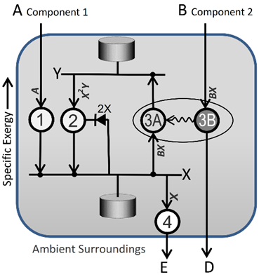
The Brusselator has four reaction nodes (circles in Figure 7–2): 1) External source A → X; 2) Y + 2X → 3X; 3) External source B + X → Y + D (discharge); and 4) X → E (discharge).
Reactions 1, 2, and 4 are exergonic transitions of component 1. An exergonic transition is a spontaneous transition to lower exergy (downward arrows in the figure). Reaction 3 is a coupled reaction, involving two separate transitions. Node 3B is an exergonic transition for component 2 from state B to state D. The component’s exergy is only partially dissipated, however. Some of the exergy is transferred to node 3A via an exergy link (wavy arrow). Node 3A is an endergonic transition. An endergonic node utilizes exergy to do work of lifting low-exergy input “uphill” to high-exergy output. The utilization of sunlight by plants to convert low-exergy water+carbon dioxide to high-exergy sugar+oxygen is a familiar example.
The Brusselator’s reaction rates, based on simple reaction rate theory and simplifying assumptions, are shown by the arrowhead expressions in Figure 7–2. At steady state, the concentrations of X and Y are fixed (triangle in Figure 7–3). For B greater than 1+A², the steady state homeostate is unstable. Any perturbation sends the system on a transient path that converges to a periodic homeostate, in which the concentrations of X and Y cycle around a stationary trajectory (Figure 7–3). The Brusselator is an example of a far-from-equilibrium system having two homeostates consistent with its boundary constaints: a steady-state homeostate and a periodic homeostate.

The Constructive Power of Dissipation
In the article, Dissipation + Utilization = Self-Organization, I proposed the Maximum Efficiency Principle as TCI’s Postulate Five:
Maximum Efficiency Principle (MaxEff): Of the multiple possibilities by which a high exergy state can transition to a more stable state of lower exergy, the transition that maximizes the conversion of energy input to work is the most stable.
MaxEff counters the effect of the Second Law of thermodynamics. The Second Law says that exergy is irreversibly dissipated, but MaxEff states that a transition seeks to defer dissipation and to maximize the conversion of energy to work. Work includes the internal work on a system’s observable parts. Figure 7–2, for example, illustrates the internal work by node 3B on 3A.
A simple example of the MaxEff is the stability of convection over conduction. Heat added to a convecting liquid does work of thermal expansion of the fluid to maintain buoyancy gradients. This is the internal work necessary to create and sustain convective flow. Heat added to a static fluid, in contrast, is dissipated by conductive heat flow, without doing any measurable work. MaxEff therefore says that if boundary constraints allow both convection and conduction, the fluid will spontaneously transition from random molecular motions to organized convective flow. This is invariably observed.
A more revealing illustration of MaxEff is the Miller-Urey experiment. Stanley Miller and Harold Urey took a mixture of simple gases and stimulated it with electrical sparks. When they analyzed the gas mixture afterward, they found that the gas molecules had reorganized themselves into a variety of amino acids. The gas mixture started in a near-equilibrium state of low-exergy. The sparks added exergy to the gas mixture, but instead of dissipating the exergy directly to heat, it deferred dissipation and utilized exergy to do work of creating high-exergy amino acids.
We can verify that the stability of the Brusselator’s periodic homeostate (limit cycle in Figure 7-3) is also related to its higher rate of internal work. The steady-state Brusselator has fixed concentrations of X and Y, but they fluctuate in the oscillating mode. The work of increasing the concentrations and exergy of the system’s component states (X and Y) during their accumulation phases is a measure of the oscillating homeostate’s positive rate of internal work. MaxEff asserts that the oscillating mode, with its positive rate of internal work, is more stable, in agreement with perturbation analysis.
We can generalize this conclusion and assert that an oscillating homeostate is more stable than a steady-state homeostate, other differences being relatively small. The spontaneous emergence of resonance, commonly observed in mechanical or fluid mechanical systems, empirically illustrates the higher stability of oscillations over steady state.
Systems of linked oscillators are often observed to synchronize in a process known as entrainment. Christiaan Huygens, the inventor of the pendulum clock, first documented this in 1666, when he observed clocks mounted on a common support spontaneously synchronize. A system of linked, but unsynchronized oscillators, can leak exergy between oscillators. This dissipates exergy and subtracts from the system’s internal work of oscillation. If oscillators are synchronized, however, there are no exergy gradients or associated dissipation, and the internal work rate increases. MaxEff provides a general principle that explains both oscillations and synchronization in terms of a general principle, independent of a system’s specific mechanics.
As a final illustration of MaxEff, we consider whirlpools. We commonly observe whirlpools, indicating they are more stable than the less organized and lower-complexity radial flow of water directly toward the drain. A simple model comparing the two homeostates shows that the whirlpool requires 4,000 times higher rate of internal work to accelerate the circulation of water in the whirlpool’s vortex compared to the much slower rate of radial flow [1].
It is commonly observed that transitioning from one dissipative process to another increases the rates of exergy supply, dissipation, and entropy production. The transition from conduction to convection clearly exemplifies this. This has led to the idea that “faster is better,” as expressed by the maximum entropy production principle and similar hypotheses. The centrifugal force of a whirlpool’s circulation, however, lowers the water level and pressure over the drain, and this actually lowers its rates of exergy supply and entropy production. The stability of whirlpools disproves maximum entropy production as a general principle. The high stability of a whirlpool results from its higher rate of internal work compared to radial flow.
The Arrows of Evolution
The simplest path to increase a system’s rate of internal work is to expand, which increases both dissipation and internal work rate. MaxEff motivates a dissipative system to increase in size or number. This defines the arrow of expansion and reproduction.
Once a system reaches its environment’s carrying capacity, it cannot expand any further. It can still increase its internal work, however, by increasing the number and interconnectedness of its network of nodes. This defines the arrow of functional complexity.
We formally define functional complexity as:
Functional Complexity = (Rate of internal work)/(Rate of Exergy input)
Functional complexity is a measurable and well-defined property of a system’s dissipative process. Convection, the oscillating Brusselator, and the whirlpool all have higher functional complexity than their less complex homeostates.
For a single pass of exergy and a single endergonic node, a system’s functional complexity can approach unity in the limit of zero dissipation and zero exergy output. However, a system can increase its functional complexity well beyond unity by reprocessing and recycling exergy via feedback loops or by sustaining a network of endergonic nodes. Feedback loops are ubiquitous within biological systems, from cells to ecosystems, leading to higher functional complexity. A stationary system with a fixed rate of exergy supply can increase its functional complexity beyond unity, with no theoretical limit.
If ample resources exist, multiple systems can proliferate and expand, increasing their number or size and rates of dissipation and internal work. For finite resources, as systems expand, at some point continued growth becomes constrained by other systems’ resource consumption. Systems then start to engage in a zero-sum competition among other systems for that resource. At some point, a system reaches its environmental carrying capacity, and further expansion ceases. Complexification and increasing functional complexity then dominates its continued evolution.
Summary
The TCI shifts physics’ focus from reversible states and transitions to stationary dissipative processes. The Second Law and MaxEff define opposing goals for a dissipative system. The Second Law guides closed nonequilibrium systems toward states of lower exergy and higher stability. This defines the thermodynamic arrow of dissipation. MaxEff guides open dissipative systems toward processes of higher internal work rate and stability. This defines the arrow of evolution. As long as an open system has sufficient resources, evolution predominates, but if the system is cut off from its resources, dissipation takes over.
MaxEff has guided the evolution of life through an interplay between Darwinian competition to increase population sizes and the internal work of reproduction, and cooperation to increase its functional complexity. The arrow of expansion drives a population of systems to its environment’s carrying capacity. Once the carrying capacity is reached, the arrow of functional complexity works at scales ranging from pre-biotic chemicals to ecosystems to increase systems’ self-organization and complexity.
[1] Crecraft, H. 2021. Dissipation + Utilization = Self-Organization. https://www.mdpi.com/1099-4300/25/2/229
[2] Crecraft, H. 2023. Time and Causality — A Thermocontextual Interpretation. https://www.mdpi.com/1099-4300/23/12/1705